Unraveling Time Series Causality with Granger Methods

This article discusses causal illusions as a form of cognitive bias and explores the use of Granger causality to detect causal structures in time series. It is common practice to analyse (linear) structure, estimate linear models and perform forecasts based on single stationary time series. However, the world does not consist of independent stochastic processes. In accordance with general equilibrium theory, economists usually assume that everything depends on everything else. Therefore, it is important to understand and quantify the (causal) relationships between different time series.

Epiphenomena

Epiphenomena is a class of causal illusions where the direction of causal relationships is ambiguous. For example, when you spend time on the bridge of a ship with a large compass in front, you can easily develop the impression that the compass is directing the ship rather than merely reflecting its direction. Here is an image that perfectly illustrates the point that correlation is not causation:

Nassim Nicholas Taleb explored this concept in his book Antifragile to highlight the causal illusion that universities generate wealth in society. He presented a miscellany of evidence which suggests that classroom education does not lead to wealth as much as it comes from wealth (an epiphenomenon). Taleb proposes that antifragile risk-taking is largely responsible for innovation and growth instead of education and formal, organized research. However, it does not mean that theories and research play no role, but rather shows that we are fooled by randomness into overestimating the role of good-sounding ideas. Because of cognitive biases, historians are prone to epiphenomena and other illusions of cause and effect.

In economic and financial time series, epiphenomena are particularly common. For instance, the relationship between interest rates and inflation often appears causal in both directions—do higher interest rates cause lower inflation, or does higher inflation prompt central banks to raise interest rates? Without proper analysis, we might misattribute causality in the wrong direction, leading to flawed policy decisions.

We can debunk epiphenomena in the cultural discourse and consciousness by looking at the sequence of events and checking their order or occurrences. This method is refined by Clive Granger who developed a rigorously scientific approach that can be used to establish causation by looking at time series sequences and measuring the "Granger cause."

Granger Causality

Granger causality is fundamentally based on prediction. The intuition is straightforward: if a variable $X$ helps predict the future values of variable $Y$ beyond what $Y$'s own history can predict, then $X$ is said to "Granger cause" $Y$. This concept, developed by Nobel laureate Clive Granger in 1969, provides a statistical framework for determining causal relationships between time series.

In the following, we present the definition of Granger causality and the different possibilities of causal events resulting from it. Consider two weakly stationary time series $x$ and $y$:

1. Granger Causality: $x$ is (simply) Granger causal to $y$ if and only if the application of an optimal linear prediction function leads to a smaller forecast error variance on the future value of $y$ if current and past values of $x$ are used.

2. Instantaneous Granger Causality: $x$ is instantaneously Granger causal to $y$ if and only if the application of an optimal linear prediction function leads to a smaller forecast error variance on the future value of $y$ if the future value of $x$ is used in addition to the current and past values of $x$.

3. Feedback: There is feedback between $x$ and $y$ if $x$ is causal to $y$ and $y$ is causal to $x$. Feedback is only defined for the case of simple causal relations.

To illustrate with an example: consider GDP growth ($x$) and unemployment rate ($y$). If including past values of GDP growth in our model helps us better predict future unemployment rates compared to just using past unemployment data, then GDP growth "Granger causes" unemployment. This doesn't necessarily mean GDP growth directly causes unemployment in the philosophical sense, but rather that it contains information useful for predicting unemployment.

Hypothesis Testing in General Linear Models

Before diving into specific Granger causality tests, it's important to understand the general framework of hypothesis testing in linear models, as this forms the statistical foundation for detecting causal relationships.

Consider the general linear model $\mathbf{Y} = X \boldsymbol{\beta} + \varepsilon$, where $\mathbf{Y}$ is the dependent variable, $X$ is the matrix of explanatory variables, $\boldsymbol{\beta}$ is the coefficient vector, and $\varepsilon$ is the error term. In hypothesis testing, we want to know whether certain variables influence the result. If, say, the variable $x_1$ does not influence $\mathbf{Y}$, then we must have $\beta_1 = 0$. So the goal is to test the hypothesis $H_0: \beta_1 = 0$ versus $H_1: \beta_1 \neq 0$. We will tackle a more general case, where $\boldsymbol{\beta}$ can be split into two vectors $\boldsymbol{\beta}_0$ and $\boldsymbol{\beta}_1$, and we test if $\boldsymbol{\beta}_1$ is zero.

Suppose $\underset{n \times p}{X} = \left(\underset{n \times p_0}{X_0} \underset{n \times\left(p - p_0\right)}{X_1}\right)$ and $\boldsymbol{\beta} = \left(\begin{array}{c}\boldsymbol{\beta}_0 \\ \boldsymbol{\beta}_1\end{array}\right)$, where $\operatorname{rank}(X)= p$, $\operatorname{rank}\left(X_0\right) = p_0$. We want to test $H_0: \boldsymbol{\beta}_1 = 0$ against $H_1: \boldsymbol{\beta}_1 \neq 0$. Under $H_0$, $X_1 \boldsymbol{\beta}_1$ vanishes and

Under $H_0$, the maximum likelihood estimation (MLE) of $\boldsymbol{\beta}_0$ and $\sigma^2$ are

and we have previously shown these are independent. So the fitted values under $H_0$ are

where $P_0=X_0\left(X_0^T X_0\right)^{-1} X_0^T$.

Note that our estimators wear two hats instead of one. We adopt the convention that the estimators of the null hypothesis have two hats, while those of the alternative hypothesis have one. This notation helps distinguish between the restricted model (under $H_0$) and the unrestricted model (under $H_1$).

The generalized likelihood ratio test of $H_0$ against $H_1$ is

We reject $H_0$ when $2 \log \Lambda$ is large, equivalently when $\frac{\mathrm{RSS}_0-\mathrm{RSS}}{\mathrm{RSS}}$ is large. Under $H_0$, we have

which is approximately a $\chi_{p-p_0}^2$ random variable. We can also get an exact null distribution, and get an exact test. The $F$ statistic under $H_0$ is given by

Hence we reject $H_0$ if $F > F_{p-p_0, n-p}(\alpha)$. $\mathrm{RSS}_0 -\mathrm{RSS}$ is the reduction in the sum of squares due to fitting $\boldsymbol{\beta}_1$ in addition to $\boldsymbol{\beta}_0$. This quantity measures how much the additional variables improve the fit of the model.

The following ANOVA table summarizes the hypothesis testing framework:

Source of var.	d.f.	sum of squares	mean squares
Fitted model	$p - p_0$	$\mathrm{RSS}_0-\mathrm{RSS}$	$\frac{\mathrm{RSS}_0-\mathrm{RSS}}{p - p_0}$
Residual	$n - p$	$\mathrm{RSS}$	$\frac{\mathrm{RSS}}{n - p}$
Total	$n - p_0$	$\mathrm{RSS}_0$

The ratio $\frac{\mathrm{RSS}_0-\mathrm{RSS}}{\mathrm{RSS}_0}$ is sometimes known as the proportion of variance explained by $\boldsymbol{\beta}_1$, and denoted $R^2$. This is a measure of how much additional explanatory power the variables in $X_1$ provide.

The following Python function implements the fitting procedure for a time series model:

def fit(data, p=1):
    n = data.shape[0] - p
    Y = data[p:]
    X = np.stack([np.ones(n)] + [data[p-i-1:-i-1] for i in range(p)], axis=-1)
    
    beta_mle = np.linalg.inv(X.T.dot(X)).dot(X.T.dot(Y))
    R = Y - X.dot(beta_mle)
    RSS = R.T.dot(R) 
    var_mle = RSS / n
    
    return beta_mle, var_mle, RSS

This function takes a time series data and a lag order p, and returns the MLE estimates of the coefficients, the variance, and the residual sum of squares (RSS). The function constructs the design matrix X by stacking the lagged values of the time series and a column of ones for the intercept.

Causality Tests

Now that we understand the general hypothesis testing framework, we can apply it specifically to test for Granger causality. The process involves fitting two models—one with and one without the potential causal variable—and comparing their performance.

To test for simple causality from $x$ to $y$, it is examined whether the lagged values of $x$ in the regression of $y$ on lagged values of $x$ and $y$ significantly reduce the error variance. By using the ordinary least squares (OLS) method, the following equation is estimated:

with $k_0 = 1$. Here, $y_t$ is the current value of time series $y$, $\alpha_0$ is the intercept, $y_{t-k}$ are the lagged values of $y$, $x_{t-k}$ are the lagged values of $x$, and $u_{1,t}$ is the error term. The first summation represents the autoregressive component (AR) of $y$, while the second summation captures the potential causal effect of $x$ on $y$.

An $F$ test is applied to test the null hypothesis, $H_0: \alpha^{1}_{12} = \alpha^{2}_{12} = \cdots = \alpha^{k_2}_{12} = 0$. This hypothesis states that the lagged values of $x$ have no effect on $y$. If we reject this hypothesis, we conclude that $x$ Granger-causes $y$.

By interchanging $x$ and $y$, we can test whether $y$ Granger-causes $x$. If the null hypothesis is rejected in both directions, we have a feedback relationship—each variable Granger-causes the other.

To test for instantaneous causality, we set $k_0 = 0$ and perform a $t$ or $F$ test for the null hypothesis $H_0: \alpha^{0}_{12} = 0$. This tests whether the contemporaneous value of $x$ helps predict $y$ beyond what the lagged values of both variables can predict.

Here's a Python function that implements these causality tests:

def causality_tests(y, x, alpha=0.05, k_1=1, maxlag=1):
    for k_2 in range(1, maxlag + 1):
        p = 1 + k_1 + k_2
        n = y.shape[0] - np.max([k_1, k_2])

        _, _, RSS = fit_xy(y, x, k_1, k_2)
        _, _, RSS_0 = fit(y, k_1)

        chi2 = n * np.log(RSS_0 / RSS)
        f = ((RSS_0 - RSS) / k_2) / (RSS / (n - p))

The function computes both chi-square and $F$-statistics for testing Granger causality. The fit_xy function (not shown) would fit the unrestricted model including both $y$ and $x$, while the fit function fits the restricted model with only $y$.

One critical issue with this test is that the results are strongly dependent on the number of lags of the explanatory variable, $k_2$. There is a trade-off: the more lagged values we include, the better the influence of this variable can be captured. This argues for a high maximal lag. On the other hand, the power of this test is lower the more lagged values are included, as we're estimating more parameters with the same amount of data.

In practice, information criteria like AIC (Akaike Information Criterion) or BIC (Bayesian Information Criterion) are often used to determine the optimal lag length. Alternatively, practitioners may test a range of lag specifications to ensure the robustness of their findings.

Application to Financial Data

We can fit a linear model on real financial data and use the Granger causality test to find causal relationships. The graph below shows a visual representation of the relationship between two financial time series:

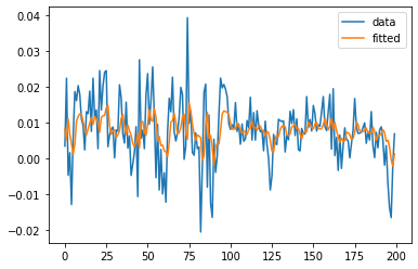
The results of Granger causality tests with different lag specifications are:

Hypothesis Test (p=1)
F test:       F=24.4610 , p=0.0000, df_denom=199, df_num=1
chi2 test: chi2=23.3023 , p=0.0000, df=1
Reject null hypothesis

Hypothesis Test (p=2)
F test:       F=8.2501  , p=0.0045, df_denom=197, df_num=1
chi2 test: chi2=8.2051  , p=0.0042, df=1
Reject null hypothesis

Hypothesis Test (p=3)
F test:       F=0.4181  , p=0.5187, df_denom=195, df_num=1
chi2 test: chi2=0.4262  , p=0.5139, df=1
Accept null hypothesis

Hypothesis Test (p=4)
F test:       F=4.9506  , p=0.0272, df_denom=193, df_num=1
chi2 test: chi2=5.0148  , p=0.0251, df=1
Reject null hypothesis

These results indicate that the null hypothesis of no Granger causality is rejected for lags $p=1$, $p=2$, and $p=4$, but not for lag $p=3$. This suggests a complex causal relationship between the two time series that manifests at different time scales. The inconsistency across lag specifications highlights the importance of considering multiple lag structures when drawing conclusions about causal relationships.

In financial markets, such findings can have significant implications for portfolio management, risk assessment, and trading strategies. For instance, if stock returns in one market Granger-cause returns in another market, this information could potentially be exploited for predictive purposes, though always within the constraints of market efficiency.