Modern Portfolio Theory

Modern portfolio theory (MPT), or mean-variance analysis, is a mathematical framework for assembling a portfolio of assets such that the expected return is maximized for a given level of risk. MPT assumes that investors are risk averse, meaning that given two portfolios that offer the same expected return, investors will prefer the less risky one.

Under the model:

• Portfolio return is the proportion-weighted combination of the constituent assets' returns.
• Portfolio return volatility is a function of the correlations of the component assets, for all asset pairs. The volatility gives insight into the risk which is associated with the investment. The higher the volatility, the higher the risk.

In matrix form, for a given "risk tolerance" $q\in [0,\infty )$, the efficient frontier is found by minimizing the following expression:

where

• $w\in \mathbb {R} ^{N}$ is a vector of portfolio weights and $\sum _{i=1}^{N}w_{i}=1.$ (The weights can be negative);
• $\Sigma \in \mathbb {R} ^{N\times N}$ is the covariance matrix for the returns on the assets in the portfolio;
• $q\geq 0$ is a "risk tolerance" factor, where 0 results in the portfolio with minimal risk and $\infty$ results in the portfolio infinitely far out on the frontier with both expected return and risk unbounded; and
• $R\in \mathbb {R} ^{N}$ is a vector of expected returns.
• $w^{T}\Sigma w\in \mathbb {R}$ is the variance of portfolio return.
• $R^{T}w\in \mathbb {R}$ is the expected return on the portfolio.

The above optimization finds the point on the frontier at which the inverse of the slope of the frontier would be $q$ if portfolio return variance instead of standard deviation were plotted horizontally. The frontier in its entirety is parametric on $q$.

An alternative approach to specifying the efficient frontier is to do so parametrically on the expected portfolio return $R^{T}w.$ This version of the problem requires that we minimize

subject to

and

for parameter $\mu$. This problem is easily solved using a Lagrange multiplier which leads to the following linear system of equations:

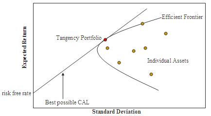
A portfolio lying on the efficient frontier represents the combination offering the best possible expected return for given risk level. The tangent to the upper part of the hyperbolic boundary is the capital allocation line (CAL).